穷乡僻壤,美丽乡村。乡党委书记是怎样使它蜕变?又用怎样的丹青勾勒出这如画风
景?
答道:以其信心,凭其决心,用其全心而已。
顿悟——人生如画,我以我心绘风景,绘出个草长莺飞,绘出个青山万丈,绘出一道
最亮丽的风景线!
我以信心绘风景,绘出一轮欲览的青天明月。五岁的她获得歌咏比赛一等奖,校长夸
奖道:“小姑娘,能拿冠军真是你的幸运。”她反抗道:“不,这是我应得的。”她是撒切
尔夫人,正是她的信心,使英国政坛多了一道迷人而又张扬的风景。
我凭决心绘风景,绘出一件已被黄沙打穿的金甲。乡党委书记凭着过人的决心建设乡
村,他成功了;孙权凭借“再有说者,便如此案”的决心,击败不可一世的曹操;邓艾凭
着“积军资之粮”的决心,以偏师平定蜀汉;项羽凭着破釜沉舟的决心,打败三十万秦
军……事例太多,但请君细想,若没有决心,曹操可能已一统天下,蜀汉仍能苟延残
喘,反秦势力可能烟消云散,那历史画卷中那些亮丽风景岂不消失殆尽?因此,我凭决
心绘风景,定要绘出“不破楼兰终不还”的豪情。
我用全心绘风景,绘出一派奋斗之花盛开的图景。乡党委书记用全心投入到乡村建
设,于是乡村焕然一新,而正值青春年少的我们,怎么有理由不全身心地投入到勾绘精
彩人生画卷之中去呢?但是,我看到了吊儿郎当的学生,我看到了沉迷灯红酒绿的青
年,他们的人生画卷黯淡无光。林清玄曾说:“我们要以全心来绽放,以花的姿态证明自
己的存在”。全心全意,只此四字,要做到却着实不易。孔明全身心地投入复兴汉室的伟
业中,即使失败也是一道风景;哈兰德•桑德斯退休后全心研究炸鸡方法,最终在街头巷
尾绘出一片“肯德鸡”的风景;科比全心练习篮球,在凌晨四点便开始训练,铸造了紫金
王朝那一抹风景。他们,或是儒生,或是老朽,或是“富二代”
,都全心投入各自坚守的
事业,亲手绘出一段段风景绚丽的人生卷轴,而我们又怎能轻易放弃?
每个人都有能力创造属于自己的风景,但需要信心、决心,更重要的是全心投入。如
此,蓦然回首,你会发现那风景已在灯火阑珊处。
我以我心绘风景,风景迷人因我心。
Cython的优化指南
很有用的资源
官方: https://cython.readthedocs.io/en/latest/src/userguide/numpy_tutorial.html
B站: https://www.bilibili.com/video/BV1NF411i74S/
基本使用
Cython可以在python中实现近似于C++的速度,基本方法是用类似于python的语法写.pyx 文件,然后再编译成python可以直接调用的library
编译需要一个setup.py
1 | # setup.py |
然后敲入入下代码就可以编译了
1 | python setup.py build_ext --inplace |
Cython还提供了很方便的visualization,可以看implementation里面有哪些是C++ 哪些是python
1 | cython -a target.pyx |
例子: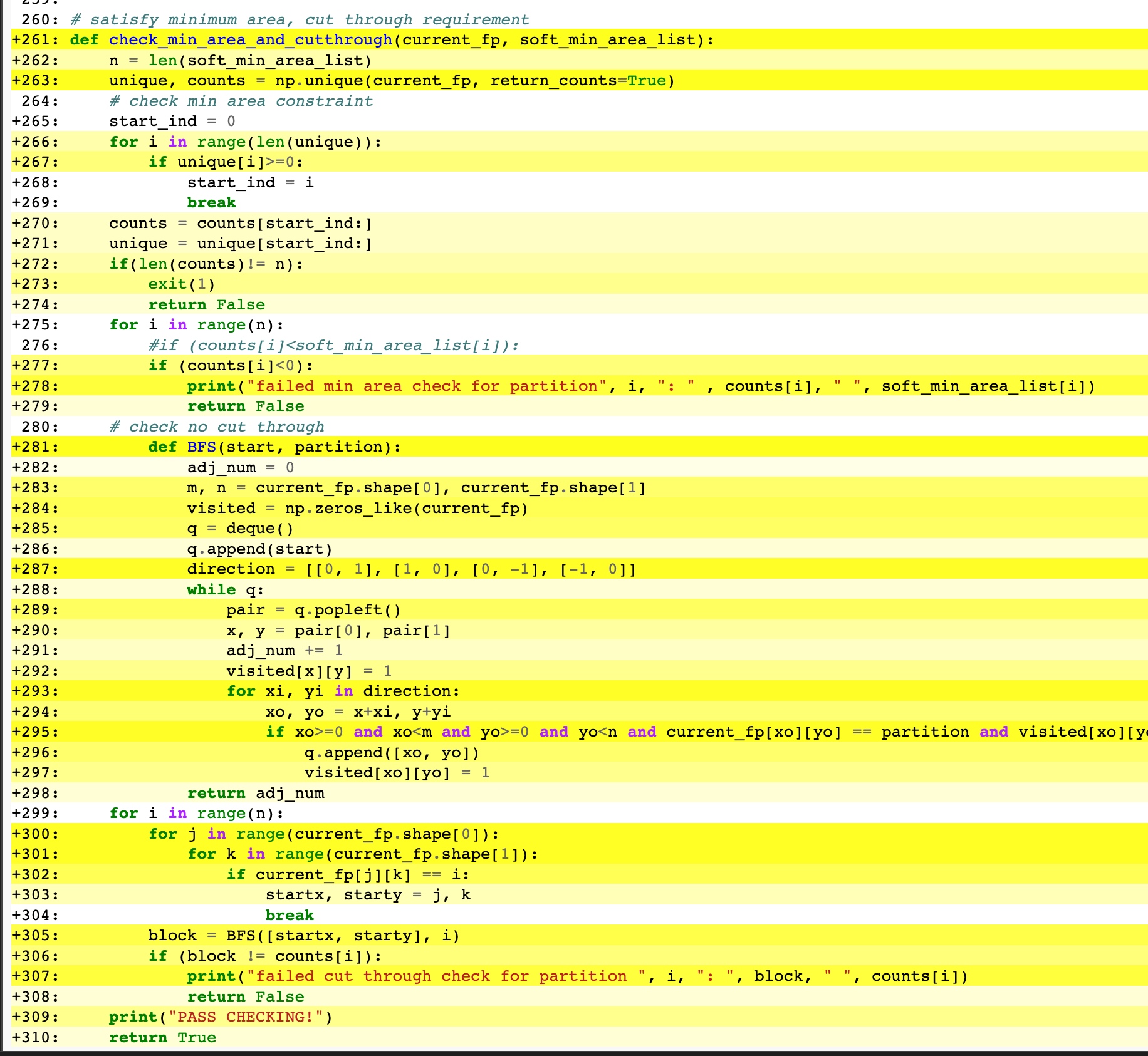
其中黄色越深,代表调用的Python API 越多,which means the efficiency is lower
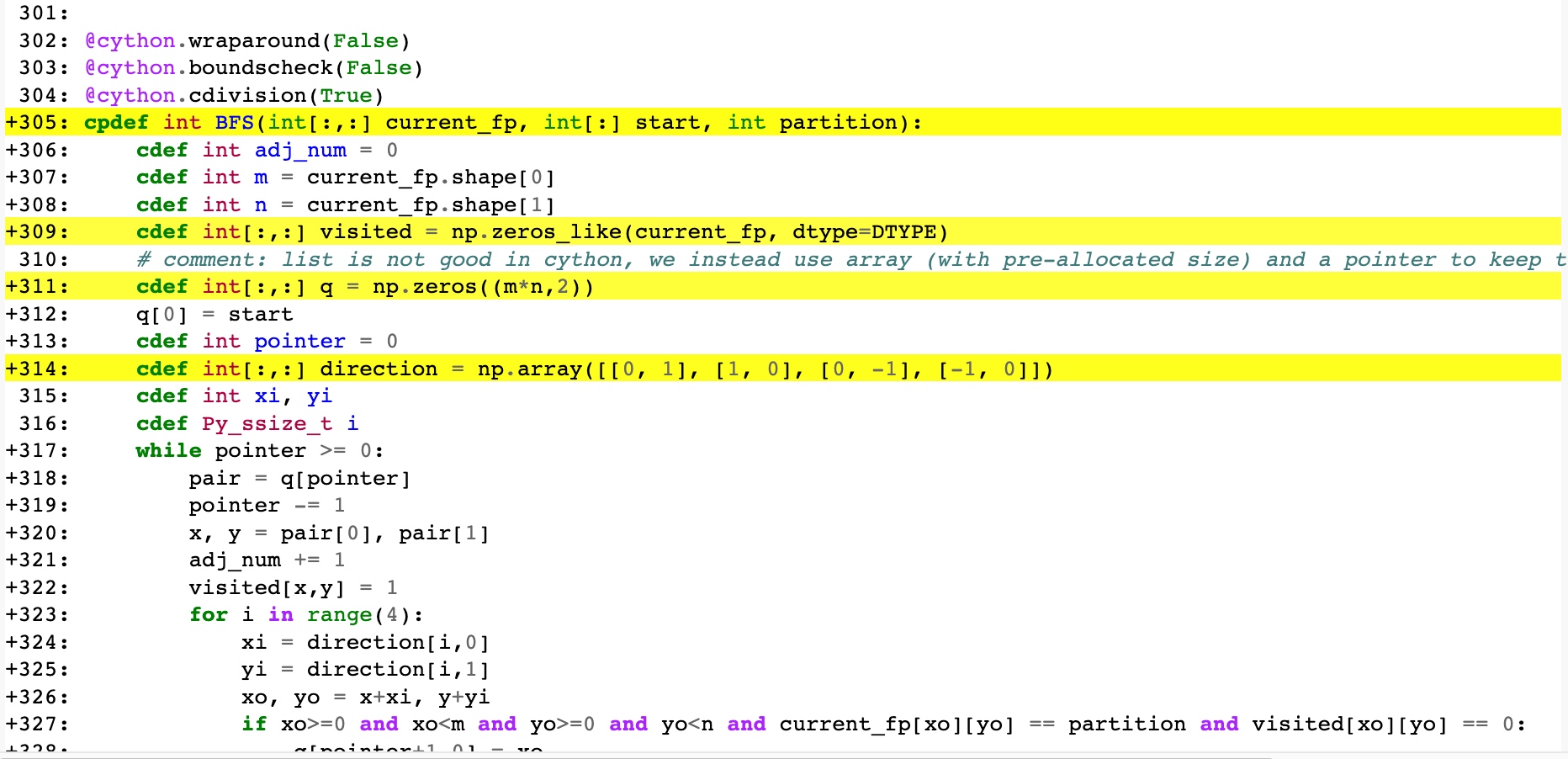
怎么优化
最常用的一般是下面几个要点
- 在function前加上
@cython.wraparound(False) @cython.boundscheck(False) @cython.cdivision(True),避免python里面耗时间的boundscheck and so on (当然这样的话bound error就不会提示了,所以建议最后没bug了再加 - 标注function input和return 的type
- 标注所有要用到的variable 的type(包括numpy array 和 index,例如i j等) (就和c一样)
- 不要直接用numpy的api,要用就自己写
效果如下,可以看到最后loop全部都白啦!
其他小技巧 OpenMP 多线程加速
在.pyx 中,加入如下prefix
1 | # distutils: extra_compile_args=-fopenmp |
然后在想要并行计算的for loop里用prange, 就可以啦:
1 | # We use prange here. |
总结
如果有些实现起来很简单,但是python因为type determine, memory allocation, bound check等 各种原因导致效率很慢,可以试着用cython来加速。效果很显著,最主要的是很容易就可以integrate into python, which is a must-have for DL work.
2024二月的碎碎念
Hey Neway.
现在是2024年的二月底。
经历了一个冬天的“匡扶汉室”后,学期一开始,我忽然有了危机感。这种感觉很像高二时候的我:就是忽然觉得自己不能再这么玩乐下去了。
也许是因为游戏玩腻了。
也许是因为DAC又中了一篇对自己要求高了一些。
也许是因为算了算自己的毕业:忽然发现四年的话就只剩一年多一点了。
一直以来我对自己说的随遇而安、开心就好的“自我安慰”的体系,似乎土崩瓦解了。
就是忽然的,我开始想work,开始算自己的paper数。
从这点上,还是蛮羡慕高中的自己的。如果下定决心,只需要心无旁骛的学习,准备高考和自主招生就行。
但是成年人的世界却不像做题考试一样简单。这样的危机感不能让我专心工作,反而带来了很多焦虑。
我焦虑自己的德不配位。焦虑自己能不能四年毕业。焦虑毕业时找教职或者找工作有没有connection能帮到我,如果没有是不是得再去多找教授合作。
德不配位这种焦虑时有发生,获得intern mentor赏识的时候;被告知Apple 很喜欢我的talk 又给了我fellowship的时候;Jose每次夸我good job的时候。当然这些时候也伴随着开心,但是开心之后就是很久的压抑。我知道自己的不足,我是个拖延症,我很多VLSI的background都欠缺,我甚至没跑个任何一个commercial EDA的flow,大学之后我也没有哪门课是真的想高中一样 感觉学到很多东西,甚至能得心应手的(天文除外)。
不过还好,这些焦虑也没有很影响到我。我觉得得学习了,那么我只需要学就好了,用不着管前路如何。到了该conection谈合作的时候,去介绍自己发email就好了。就像小撒说的
“我觉得自己是自由的。我不给自己的明天设置任何目标。我完全让时间这条河流带着我往前走,我就像躺在河面上的孩子一样,河流到哪,我就到哪,我只看天上的白云,不看前面”
我经常会庆幸自己喜欢历史、也算“饱读过诗书”,所以这些压抑的负面的情绪,基本也都能消遣掉。竹杖芒鞋轻胜马,谁怕?一蓑烟雨任平生。
我很喜欢回过去看自己写的碎碎念。这真给了我一种穿越时空对话的感觉,同时很多时候也给了我无穷的精神力量。我想,未来某个时候的你,看到这篇文章,也会重温苏子当年给你的激励,也许也能帮你排解一些忧愁。
真好。
Survey of VLSI LLM
| Category | Base Model | Data | Open-source | Training cost | Problem | Metric | Experimental Conclusions | Other Remarks | |
|---|---|---|---|---|---|---|---|---|---|
| DATE23-BPAN, Benchmarking LLM for automated Verilog RTL Code Generation | Fine-tuning | CodeGen, 345M - 16B | Github: 50K files / ~ 300MB: Verilog Book: 100MB | Yes | CodeGen 2B: 1 epoch, two RTX8000(48GB), 2days; CodeGen 6B: 1 epoch, 4 RYX8000(48GB), 4 days; CodeGen 16B: 1 epoch, 3 A100, 6 days. | Code generation from HDLBits website | 1. Compiled completions; 2. functional pass | 1. Fine-tuning increase compiling completion rate significantly; (with 10 different completions) 2. Fine-tuning is still bad at functionality correctness of intermediate and advanced problems | LLM is only good at small scale/ light-weight task |
| ChipNemo | Fine-tuning | LLaMA2, 7B, 13B, 70B | Internal Data (Bug summary, Design source, Documentation, verification, other): ~22B tokens; Wiki: 1.5 B tokens [natural language]; Github: 0.7 B tokens, C++, Python, Verilog [code]. | No | 7B: 2710 A100 hours; 13B: 5100 A100 hours | Script Generation; Chatbot (88 practical questions in arch/design/verification); Bug summary and analysis | Mostly human rating | A lager lr. (3x10e-4 vs5x10e-6) degrades performance significantly | In most cases, 70B w.o. FT is better than 13B w. FT |
| ChatEDA | Fine-Tuning | LLaMA2, 70B | In-context learning (give example in prompt) gives 1500 instructions + proofreading. | No | 15 epochs, 8xA100 80GB, | task planning; Script generation | 1. the task planning is accurate? 2. the script generation is accurate? | Auto-gressive objective? | |
| RTL-Coder | Fine-Tuning | Mistra-7B-v0.1 | 27k+ samples (pair of problem + RTL code ) | Yes | 4 RTX4090 | RTL code generation | VerilogEval + RTLLM | The new training scheme seems to be very effective; Using generation method in RTLLM, the function correctness even reaches 60% for GPT4 |
我和三国的故事
初中时我的历史和地理特别好,好到基本没有下过一百分。很大一部分原因是因为兴趣吧。至今我都还清楚记得一个画面:周末午后的暖阳下,我躺在躺椅上惬意的读着各种历史地理的科普书、小说。
其中便有三国演义。不过当时稚嫩的我,只是纯粹把它当作一本“描绘英雄的故事书”。当时的我喜欢是无所不能的诸葛亮、是七进七出的赵子龙、是一个又一个豪迈的英雄故事。就像对迪迦的迷恋一般,我和大多数少年一样,是崇拜并且深信这些英雄的:无论何时,他们都会像光一样,而这个世界,也会无偿的相信支持他们的英雄,最终,英雄会打败邪恶,拯救这个世界。
也许是从大学开始,慢慢的需要接触社会、面对除考试外的压力、承担作为成年人的责任,我认识的似乎更深刻无情了一些。这个世界上没有奥特曼也没有英雄,只有努力却不一定成功的人。诸葛亮不会呼风唤雨、子龙也没有七进七出(当然他确实在长坂坡救了阿斗)。这些“英雄”们的生活,其实也充满着一地鸡毛:几万士兵粮食哪里来,拉屎拉哪里,新兵蛋子去偷橘子了怎么办,家里老婆孩子又生病了怎么办。。。
但反而如此,我却更加喜欢蜀汉的这群人了。
读到司马懿的“洛水之约”,我越发倾佩丞相身居高位却真正做到了“鞠躬尽瘁死而后已”。
看到曹操每过屠城,我也更喜欢那个携民渡江“吾不忍也”的刘玄德。
只有自己在人生选择中做了太多次的“精致利己者”,才会感慨姜维“可使汉室幽而复明”那“明知不可为而为之”的胆量与魄力。
我相信权力场不只有尔虞我诈;我相信即便成功渺茫,我们也可以尽力一试;我相信人际关系不是只讲利益。我相信这些,不是因为我自己的感同身受,不是因为课堂上学到了这些,而是因为我知道,一千八百年前,有这么一群理想主义者,无论成功与否,他们真的是这么做的。
几千年的滚滚长河,无数王侯将相化为尘土,我只感到何其有幸,能读到他们的故事。每每失意之时,他们便在我心中似乎真化作了光,指引我前进的方向,并激励着我一路前行。
DAC23之后的一些碎碎念
Hey Neway, 现在是加州的凌晨0点22分,度过了一周的DAC,本来应该困顿的我现在特别清醒。所以干脆还是写点什么记录一下这次DAC。
该死的疫情总算死了,我也得以见到好多在香港时的好友。有些人似乎没有变、有些人却经历了一些难过和挫折。每当有这些负面经历时,我都会安慰自己:就当是一种人生新体验好了。但是对他们我却不太会拿这个原因来安慰他们,我只是和他们一样觉得难过、觉得惋惜,同时也觉得人生的残酷:它永远这么长河般的向前流、而平凡的我们却很难做那个掌舵手、只能被岁月推着往任意方向前行。
很擅长optimization的我们,貌似很难optimize我们自己的人生,哪怕只是一点点。
说回这次DAC吧。Presen的时候感觉自己还是因为紧张 说的太快了,之前在Apple的时候Mark就给我建议presen前深呼吸、注意自己的语速。结果我只记得上半句,诶。不过除了说了快一点、公式放的有点多之外,其他的似乎一切都好,我也不知道什么时候,好像有了《哪怕紧张 也会“看起来”很自信》的天赋,挺好的。确实得自信一点,这是自己的work,自己几个月的心血,自己都没底气的话,那也太对不起work的那个自己了吧。
线下的这种会议对于开拓眼界真挺有用的。感觉这几天看到的EDA、PD比我过去一年看到的都多:从前一直都像是盲人摸象般,而在这能去到不同的session、能了解各个组最新的work,这种机会不是arxiv、google scholar看paper能比拟的。虽然无法避免的会有一些peer pressure,但是更多的还是感悟、学习、和收获吧。
BTW。这次还见到了许多paper里才看得到的老师,真有点像小虾米第一次参加武林大会时见各个门派的掌门的感觉哈哈哈哈。从这个角度看学术圈还真挺像武侠世界的。那些很有影响力的paper时降龙十八掌、六脉神剑、而我发的paper暂时还只是“花拳绣腿”、“王八拳”,哈哈。(那去公司是不是就是去镖局之类的上班 XD
每次写这种文章的时候,我都会打开Hey Kong单曲循环。我也好想知道未来的你在做什么,想听到未来的你对我说的话。但不管怎样,希望你和大家都能一切如意。
德州的记忆
Mark夸我做得好
| Original | Correction | Reasoning |
|---|---|---|
| Central to my research interests are optimization and GPU-accelerated methods in VLSI design and test, as well as geometric deep learning and its applications in EDA. | My primary research interests lie in optimization, GPU-accelerated techniques in VLSI design and testing, alongside geometric deep learning and its applications in Electronic Design Automation (EDA). | Clarification and enhanced readability. |
| My research endeavors have culminated in over a dozen publications, including three best-paper awards. | My research efforts have resulted in over twelve publications, including three papers recognized as best in their respective categories. | Improved sentence structure for clarity. |
| Chiplets, exotic packages, 2.5D, 3D, mechanical and thermal concerns, gate all around, …, make the already-hard problem of IC design that much more challenging. | The incorporation of chiplets, exotic packages, 2.5D, 3D integration, as well as mechanical and thermal considerations, alongside emerging technologies like gate-all-around (GAA), exacerbate the already complex nature of IC design. | Enhanced clarity and precision. |
| Existing CPU-based approaches for design, analysis, and optimization are running out of steam, and simply migrating to GPU enhancements is not sufficient for keeping pace. | Traditional CPU-based approaches for design, analysis, and optimization are becoming inadequate, and a mere transition to GPU enhancements is insufficient to maintain pace. | Improved phrasing for academic style. |
| New ways of solving both existing and emerging problems are therefore desperately needed. I am very much attracted to these types of challenges and take pleasure in generating solutions that exceed old techniques by orders of magnitude. | There is an urgent need for innovative solutions to address both existing and emerging challenges. I am particularly drawn to these types of problems and find satisfaction in devising solutions that surpass previous methods by significant margins. | Strengthened expression of urgency and motivation. |
| In collaboration with Stanford University, my lab at CMU developed a new testing approach for eliminating defects that led to silent data errors in large compute enterprises \cite{li2022pepr}. Our approach involved analyzing both the physical layout and the logic netlist to identify single- or multi-output sub-circuits. The method is entirely infeasible without using GPUs, which allows us to extract more than 12 billion sub-circuits in less than an hour using an 8-GPU machine. In contrast, a CPU-based implementation required a runtime exceeding 150 hours. | In collaboration with Stanford University, my lab at CMU devised a novel testing methodology to rectify defects responsible for silent data errors in extensive compute infrastructures \cite{li2022pepr}. Our approach entailed scrutinizing both the physical layout and logic netlist to pinpoint single or multi-output sub-circuits. This method is entirely unattainable without the use of GPUs, enabling us to extract over 12 billion sub-circuits in under an hour using an 8-GPU system. In contrast, a CPU-based implementation demanded a runtime exceeding 150 hours. | Enhanced clarity and precision. |
| My summer intern project concerning global routing at NVIDIA\footnote{Submitted to IEEE/ACM Proceedings Design, Automation and Test in Europe, 2024} is another example to demonstrate. Specifically, traditional CPU-based global routing algorithms mostly route nets sequentially. However, with the support of GPUs, we proposed and demonstrated a novel differentiable global router that enables concurrent optimization of millions of nets. | My summer internship project focused on global routing at NVIDIA\footnote{Submitted to IEEE/ACM Proceedings Design, Automation and Test in Europe, 2024} serves as another illustration. Conventional CPU-based global routing algorithms predominantly route nets sequentially. Nonetheless, with the aid of GPUs, we introduced and demonstrated an innovative differentiable global router that facilitates simultaneous optimization of millions of nets. | Improved phrasing for academic style. |
| Motivated by my intern project at Apple in 2022. Unlike traditional floorplanning algorithms, which heavily relied on carefully designed data structure and heuristic cost function, I first proposed a Semi-definite programming-based method for initial floorplanning, which is a totally new method and outperforms previous methods significantly \cite{10247967}. Furthermore, I designed a novel differentiable floorplanning algorithm with the support of GPU, which is also the pioneering work that pixelized the floorplanning problem. | Inspired by my internship project at Apple in 2022, I introduced a fundamentally new approach to initial floorplanning. In contrast to conventional methods, which heavily depend on intricately crafted data structures and heuristic cost functions, I advocated for a Semi-definite programming-based approach that exhibits superior performance \cite{10247967}. Additionally, I devised an innovative differentiable floorplanning algorithm with GPU support, marking a pioneering effort in pixelizing the floorplanning problem. | Enhanced clarity and precision. |
| While Artificial Intelligence (AI) has witnessed resounding triumphs across diverse domains—from Convolutional Neural Networks revolutionizing Computer Vision to Transformers reshaping Natural Language Processing, culminating in Large Language Models propelling Artificial General Intelligence (AGI)—its impact on the IC domain has been somewhat less revolutionary than anticipated. | Although Artificial Intelligence (AI) has achieved remarkable success in various domains—from the revolutionizing effects of Convolutional Neural Networks on Computer Vision to the transformative impact of Transformers on Natural Language Processing, culminating in Large Language Models propelling Artificial General Intelligence (AGI)—its influence on the IC domain has been somewhat less groundbreaking than anticipated. | Strengthened expression and enhanced precision. |
| This can be attributed, in part, to the irregular nature of elements within the VLSI workflow. Notably, both logic netlists and Register Transfer Level (RTL) designs inherently lend themselves to representation as hyper-graphs. Moreover, the connectivity matrix among blocks, modules, and IP-cores is aptly described by a directed graph. Unlike the regularity found in images or textual constructs, the application of AI to glean insights from such irregular data remains an ongoing inquiry. | This can be attributed, at least in part, to the irregular nature of components within the VLSI workflow. Notably, both logic netlists and Register Transfer Level (RTL) designs inherently lend themselves to representation as hyper-graphs. Furthermore, the connectivity matrix among blocks, modules, and IP-cores is aptly described by a directed graph. In contrast to the regularity found in images or textual constructs, the application of AI to extract insights from such irregular data remains an ongoing area of exploration. | Enhanced clarity and precision. |
| My prior investigations into layout decomposition \cite{li2020adaptive} and routing tree construction \cite{li2021treenet} vividly underscore the immense potential and efficacy of geometric learning-based methodologies in tackling IC challenges. | My previous studies on layout decomposition \cite{li2020adaptive} and routing tree construction \cite{li2021treenet} strongly emphasize the significant potential and effectiveness of geometric learning-based approaches in addressing IC challenges. | Improved phrasing for academic style. |
| A recent contribution \cite{li2023char} of mine delves into the theoretical boundaries of Graph Neural Networks (GNNs) in representing logic netlists. Drawing upon these foundations and experiences, my overarching research ambition in my PhD trajectory is to develop the Large nelist model to capture the function information of logic netlist |
2023年六月的随笔
Forbidden area!
Install PyG under Arm Mac
- Install nightly pytorch:
1
pip3 install --pre torch torchvision torchaudio --index-url https://download.pytorch.org/whl/nightly/cpu
- Install these packages from the source:
1
2
3
4
5pip install --no-cache-dir torch==1.13.0 torchvision torchaudio
pip install git+https://github.com/rusty1s/pytorch_sparse.git
pip install git+https://github.com/rusty1s/pytorch_scatter.git
pip install git+https://github.com/rusty1s/pytorch_cluster.git
pip --no-cache-dir install torch-geometric
Advantages of ReLU
STRATEGIES FOR PRE-TRAINING GRAPH NEURAL NETWORS
Motivation: Naïve pre-training strategies (graph-level multi-task supervised pre-training) can lead to negative transfer on many downstream tasks.
Pre-train Method
NODE: Context prediction:探索graph structure information
context graph: for each node, the subgraph between $r_1$-hop and $r_2$-hop.
context anchor nodes: 假设GNN是r-hop,context anchor nodes就说context graph和r-hop overlap的点。(也就是r1 到 r 之间的点)
- 获取context embedding
- 用GNN获取context graph 上的node embedding
- average embeddings of context anchor nodes to obtain a fixed-length context embedding.
- context embedding和对应的r-hop 的node embeeding的inner product接近1 (prior that the two embeddings must be similar when they come from the same neighborhood)
NODE (also applies to GRAPH level): Mask attributes and predict them
Principal Neighbourhood Aggregation for Graph Nets
单个aggregator不行,需要combine多种不同aggregator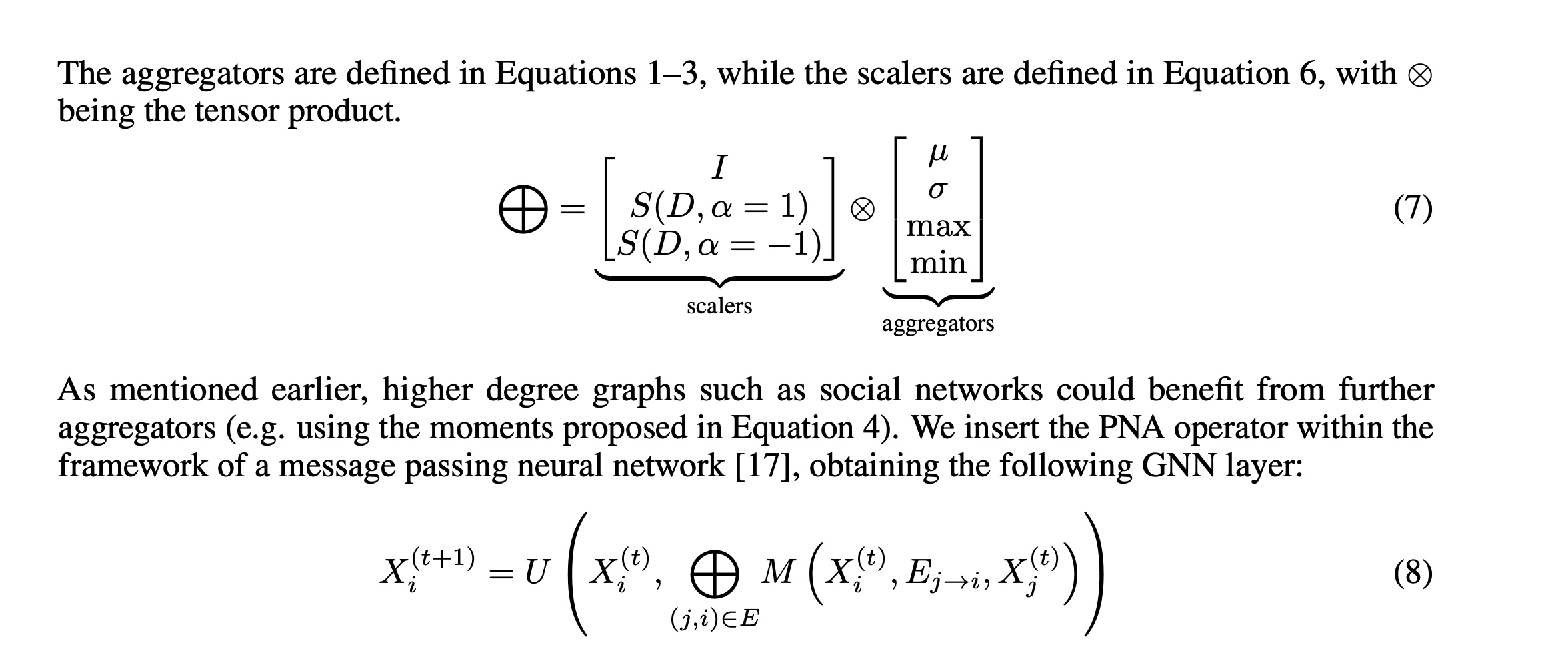
这里的S 是基于degree的一个额外系数: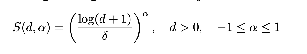
alpha pos时,node的degree(d)越大,S值就越大,于是feature值越大。(amplification)
反之则为 attenuation
Global Self-Attention as a Replacement for Graph Convolution
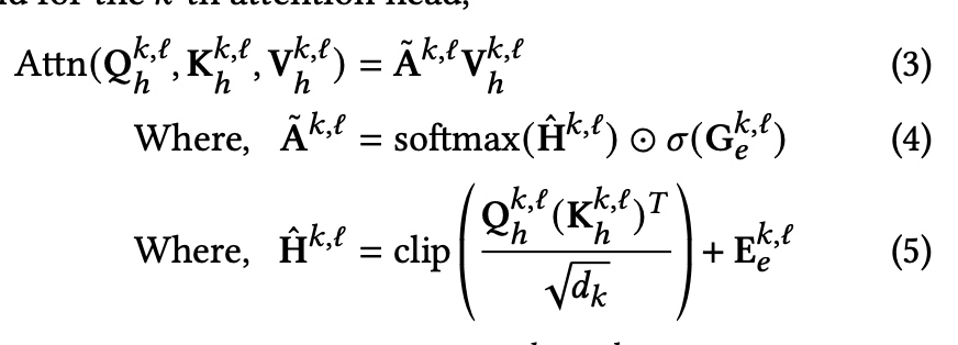
The basic idea is, rather than pre-defined functionality of edges, which introduce inductive bias. Let transformer learns it by itself.
here, edge information used in:
- $G$ is linear projection from edge embeedings. Will be a gate contriolling the attention. (Eq 4)
- $E$ is a linear projection from edge embeddings. Directly influence attention. (Eq 5)
- $E$ SVD on adj mat A, and use left and right singular vectors as positional encoding.