0%

STRATEGIES FOR PRE-TRAINING GRAPH NEURAL NETWORS

Motivation: Naïve pre-training strategies (graph-level multi-task supervised pre-training) can lead to negative transfer on many downstream tasks.

Pre-train Method

NODE: Context prediction:探索graph structure information

context graph: for each node, the subgraph between $r_1$-hop and $r_2$-hop.
context anchor nodes: 假设GNN是r-hop,context anchor nodes就说context graph和r-hop overlap的点。(也就是r1 到 r 之间的点)

  1. 获取context embedding
    1. 用GNN获取context graph 上的node embedding
    2. average embeddings of context anchor nodes to obtain a fixed-length context embedding.
  2. context embedding和对应的r-hop 的node embeeding的inner product接近1 (prior that the two embeddings must be similar when they come from the same neighborhood)

NODE (also applies to GRAPH level): Mask attributes and predict them

Principal Neighbourhood Aggregation for Graph Nets

单个aggregator不行,需要combine多种不同aggregator

这里的S 是基于degree的一个额外系数:

alpha pos时,node的degree(d)越大,S值就越大,于是feature值越大。(amplification)
反之则为 attenuation

引言

科学是一个继承与积累的过程,强如牛顿世不是一个人发展动力学、一个人收集整理数据!(Cohen 62) ,然而从牛顿运动定律到达尔文的自然选择学说,再到爱因斯坦的相对论原理 ,每次新理论的出现现往往伴随随对前人科学的否定。

本文将从探讨几位科学巨匠的继承与叛逆入手,分析继承与叛逆在科学的发展中所扮演的角色,从而思考其能给我们带来的启示。

科学巨匠们的继承与叛逆

牛顿

谈到科学史,牛顿是绕不开的话题。牛顿《自然哲学中的数学原理》《以下称《原理》)的问世是整个物理学史中最伟大的事件之一(Cohen 49),而牛顿也被公认为将科学与宗教分离的现代科学开创者(陈方正 595)。在后人看来,对于那个以亚里士多德体系为科学标准的时代,牛顿可以说是以叛逆者的形象出现的。而这点恐怕是牛顿万万没想到的,事实上,无论是在宗教层面曾用天体运动证明神的存在(Cohen 55)还是在数学层面对于古典几何学的发扬,牛顿都是一个古代传统的继承者而非叛逆者,这也与其本人想法一致(陈方正595)。

牛顿的自诩不无道理。现代科学革命是由古希腊科学的复兴所触发(陈方正628),牛顿的科学体系也有许多是继承了古希腊科学思维。牛顿在无数例子中提炼出了惯性定律,而古希腊科学也重视演绎和归纳,譬如试图将地、海、火、风这些常见的自然现象感景观归纳为构成世界的四种元素(Lindberg 27)。《原理》对定理的证明逻辑严密,对数学的运用也十分巧妙,这些也正符合古希腊科学的特征(Thomas 89)。

但仅将牛顿称为继承者又显不妥,牛顿的许多贡献,如微积分、实验科学是超出了前人的研究程度甚至理解能力的,而这些贡献又一定程度上颠覆了前人的科学体系或是思维方式,这也是牛顿会被大众视为“叛逆者”的原因。但我认为,牛顿的最好定义应当是继承者、发展者和叛逆者。一方面,牛顿继承了前人部分思维方式、吸收了同时代其他科学家们的实验或是理论结晶,最后发展出将数学、观测、思想三者系统的结合起来的崭新哲学(余英时),而这门哲学反过来颠覆了传统理论,即叛逆一说。

达尔文

作为另一个叛逆者的杰出代表,达尔文的叛逆显而易见,他认为自然选择使产生有利变异的个体有更好的机会生存并将这个有利变异遗传下去,而有利变异的逐步积累则产生了物种进化,后来便出现了人类这样的高等生物(Darwin 95),这对上帝造人说无疑是巨大的挑战。

事实上,达尔文不仅是个叛逆者。他分别吸收了莱尔地质缓慢变化理论,马尔萨斯的资源有限导致生存竞争的概念·拉马克的特征可传理论,并将三者结合起来,再联系自己的实验及理论最终形成了自然选择学说。

坎德尔

作为当代科学家的杰出代表,坎德尔的研究历程更值得深思。他不是以“叛逆者的形象出现,而是一位优秀的合作者,继承者。

在探索意识的生物学基础这个尚未有人“开发”的难题时,他的导师建议他从下而上研究神经细胞的内部世界进而探索更上层的心理结构理论(Kapde1180),而在探索负责意识统一性的分布位置时巨匠克里克给了他关于屏状核的启示(Kandel 190)。可见人类的知识已不可能由一个人来全方位的扩展,当代科学中多人合作已不可避免。

分析

如上,达尔文的历程与牛顿都经历了吸收他人理论、发展自己理论、推翻前人理论的过程。但两人本意并不是叛逆,他们只是在发展自己的理论后发现与传统理论矛盾,于是选择成为叛逆者推翻原有理论。

用一个比喻来说明继承、叛逆与发展在科学中的角色:将科学比作一张试卷,继承就像试卷前面的基础题,你只需学习前人的理论便可,而发展就像是后面没有标准答案的难题,你得推导出更深层次的理论才可能完成。叛逆的一部分是你推导理论时跳出前人知识圈子的能力,而当你做完后面的难题,得到了自己的理论,发现基础题根本不能按从前的方法做时,你冒着 0分的风险把基础题全改掉的勇气就是叛逆的另一部分。

至于当代高层次的科学,就好像是几个人一起做一张只有难题的试卷,大家各抒已见,互帮互助,互相吸收时方的思路,这是发展。而一张卷子用了好几代人的时间来做,后人看前人的思路来继续解题,这是传承。当后人发现的人的思路有问题一笔涂掉,这是叛逆。当然,最后卷子做完,这张卷子的题目以后就变成基础题等着后人来做了。

启示

对于我们学生来说,继承无疑是容易的,但发展则困难些,它需要我们去探索未知的可能,而叛逆则更显困难,因为我们首先需要一套严密的体系去推翻它,这需要有足够的知识,而学习时我们又得小心不要陷在原体系的思维局限中,这无疑更为困难。因此在学习时锻炼自己的思辨能力以及敢于犯错的能力是及其重要的。

但同时,我们也不能盲目叛逆·不顾前人已得到的经验而盲目的追求标新立异、妄图空想出一个改变整个科学历史的重大发现自然是不可取的。从牛顿到达尔文,没有一个不是在学习、实验无数小时、自成了一套严谨科学的体系之后才开始叛逆,尚不能行,焉能跑否?这在当代的科学环境中尤为重要。

相对叛逆,我们更应思考如何在继承的基础上发展知识。细说,我们在将目前的课程掌握的基础上可以把握大学广淘的资源,去深入探索更高层次的问题,广说,谁也不能断言爱因斯坦构建的物理大厚不会崩塌,但我们能确信的是科学将会一直发展,我们能做的就是学到人类知识边缘,然后以团队之力为科学开疆扩土,并将这份志愿传承下去。

总结

克里克说,如果他可以活得久一些,他就要做一个实验确认当某个刺激进入意识知觉时,屏状核是否被激活了。他没有完成,但他的思路给了后人启示,于是坎德尔完成了。这种科学家之间的传承,何尝不令人动容?

历史上那些对科学的发展做了贡献的科学家们,就如已演变成中子星但仍在浩静夜空中闪耀着光芒的恒星的“鬼”,即使已经消亡,但星光一直在照耀我们。

若我们在黑夜里寻求真理时能有一缕星光相伴,即使可能会走弯路,总比闭着眼往前走来得可靠得多。而当我们走到一片完全没有星光的黑夜之中时,我们大可以毫无顾忌的摸索前进,因为终究有一天,会有一个执着着摸索前进着的人,成为这片黑夜上的星光给之后前来探路的人照亮前路的方向。

未来,当你再次仰望星空,看到这些可能几百万年前便已逝去但仍将光辉抚在你脸上的繁星,你想到亚里士多德,想到牛顿,想到达尔文,斯人已逝,科学犹存,这也许就是科学的魅力所在。

而我们擎路蓝缕,如坎德尔继承克里克一般,头顶星光脚踏实地的不断探索先人未曾或未能触及的领域,这也许就是对继承与叛逆最好的注解。

这篇文章作于2015.04,是我与自然对话的Final paper。转眼便是八年,我也真的在做一些算是“新东西”的科研,每每再读,都思绪万千。希望自己的赤子之心不要随着时间磨灭,希望自己能真的脚踏实地,有幸也能成为漫漫黑夜中的那一束星光。

写完这个文章 发现自己的文学功底退化的十分明显。但又能怎么办呢,时间把我的才华偷走了。

关于这篇floorplan的那些事

这个work的整个过程真有点哲学意味:
本来想的是投一篇apple做的work,结果apple不给数据,
反而是在那个work中发现了一个子问题自己捣鼓出了这个work;
捣鼓完paper结果因为系统钓鱼执法不能提交了,
其实那时候心里已经想着烂掉了,就这样吧,但不知道为什么还是坚持“骚扰”了chair两三次,最后还是交上去了。
人生哪,永远不知道下一粒巧克力是什么味道,但是如果不去尝一下,那就永远都不知道下一粒没准是提交成功并且accepted的“惊喜”呢。
就像Jose说的

Fantastic. Persistence wins.

尽吾志也而不能至者,可以无悔矣。“可以无悔”重要,“尽吾志也”也很重要。

paper的规划

来CMU前,我定下了一个看起来很完美的五年计划

  • 每年 中 一篇paper
  • 每学期 投 一篇新paper

计划有条不紊的进行,现在也是达标的状态。但我忽然发现一个问题:
如果每年中一篇,但是每学期投一篇,那岂不是意味着最后我会有一半的投稿都跟我的coloring一样去arxiv了?
emmm。。。

方向

认识了一些人、投了这么些paper后,发现方向实在是太重要了。
虽然其实不同方向需要的数学方法都大同小异,但是
发paper、找教职、拉funding看的不是你数学能力、实现能力、思维能力,还得看你的方向match不match。
说到这个我就头大了。
之前说过,感觉自己只是一个天马行空的铺水泥的,缺少一个建筑师该有的大局观。
也许我需要多学习、多思考、多交流、多聆听,才能找到那个方向吧。

三国志14

之前沉迷三国志14的时候,因为对游戏中的数值设定不满,于是自学了CE,然后自己调了一些数值,并且发到了网上。
最开始一两天没有掀起什么波澜,甚至连回复的也没有。我本来挺失落的:第一次游戏编程 就这么结束了,一点水花都没掀起。
结果过了半年多,那个帖子火起来了,下面一堆“大神”、“大佬“的留言差点没让我迷失自我。
甚至还有一个初中生通过手机号加到我的微信,出钱让我帮他改数值,哈哈。
每次疲倦重复每日工作、会议的时候,想到这些,才会有种自己是真的在生活的感觉。真好呐。

我记得

这是我最近单曲循环的一首歌。
本来只是觉得曲子好听,直到听到这句词:

在星空另一端 思念从未停止 如同墓碑上的名字

然后就没法阻止的想到了高武。
想到当年他给我小姨发短信说我心情不好让小姨多照顾我;
想到他瞒着我偷偷给我妈汇报我最近的心情、学习;
想到高三最后两个月和他在被子里一起偷听他喜欢的电台;
想到大学后他在qq上给我的留言:李巍,你最近过的怎么样;
想到知道他去世时候我哭到站不起身;
想到去他家里他爸孤身一人家徒四壁的情境。
也许另一个时空,我仍和他互为挚友,回国时也会去找他把酒言欢。
但是我这个时空他永远的离开了,人世间这么精彩,但是高武已经只剩一个墓碑,永远孤零零的在那大山里了。
不过我相信,就像三体中说的,刻在石头上的信息往往比现代科技存储的更久。
高武的墓碑肯定会一直在那,就像我对他的思念一样。

因为实习太累,所以昨晚睡得很早,到了凌晨迷迷糊糊的反倒睡不着了。既然睡不着,便起床把一些要处理的工作顺手完成,然后吞了一粒褪黑素,继续躺床上,大脑反而越来越清醒。

不行啊,明天可不是周末,还有各种会要开。

本来想找本书看,但是又没带kindle或者什么书来加州。寻思了一会,既然读不了,干脆就随便写写。

人类的寿命一般是75岁左右,所以我的人生也在今天正式走过了三分之一的旅程(如果顺利活到75的话)。三分之一不是一个小数字了,比如什么task的accuracy只有66.7%的话,我大概率会觉得这个算法很水:有三分之一的样本都搞错了,有啥厉害的。

有三分之一的时间都很无趣的过去了,有啥厉害的。

是的,回过头看自己三分之一的人生,好像并没有值得说道的地方。世界上有那么多有意思的事、有意思的地方、有意思的美食等着我去尝试,但是我探索过的太少了。过去的这二十几年,感觉自己一直都活的很仓促。好像都有双无形的手在推着我前行,高中要搞奥赛、高考,大学后面要计划未来,然后MPhil要看paper考托福申请,到了PhD还要看paper写paper,哪怕来到加州也是各种各样的会议、deadline等着我去fulfill。年纪越大,时间仿佛就过的越快,也越来越多的希望自己能让时间停下来:这样我就可以把这个paper写完了/这样我就可以把这个实验跑完了/这样就可以。。。即便是自己的幻想中,我也只是希望自己能有足够的时间去工作,而不是有一点点时间可以停下来享受生活。

时间的长河看不到尽头 像只鱼儿游没办法逆流

这就是一个很多人都熟悉的矛盾点:小时候有时间有精力,却没钱没vision(视野?);大了有钱了知道自己喜欢什么想做什么了,却没时间了。

不过真要说起来,我对这三分之一的人生倒是很知足了。

我有太多受之有愧的恩赐了。这世上有太多在经历生老病死的人、有太多还在为生计发愁的人、有太多没有出过国、没有机会接受高等教育的人,大家不都还在努力的生活着吗。我现在的消愁,跟真正还在泥潭中挣扎的人来比,只能算得上是“为赋新词强说愁”吧。

PS:塞尔达

一个阶段性的总结

HI Neway。hou nai mo giai!现在是加州的晚上11点,不像香港的湿热、湖南的变幻、匹兹堡的阴沉,加州的太阳特别好,每次骑单车出门时都会被那恰到好处的阳光惊艳到,然后有种想立刻出去hiking的冲动。我也算理解为什么那么多人都说加州比匹兹堡好多了。

我想我需要回顾下过去半年、或者来CMU的一年发生了什么。之前说要投两篇paper:最终还是做到了——虽然又做了一次deadline fighter,写作质量什么的也无法顾及。

能力 想做的

其实我对自己的状态是挺不满意的。

大概来说,感觉自己是个“心比天高”却又“力比纸薄”的人物。我有好多想做的,但是自己的能力却又跟不上这些志向。

要学的 想学的 眉毛紧锁 焦虑

人生海海

至少快乐伤心是我自己决定

This is a reading notes for recipe generation papers, whcih is for my 10701 projects.

Generating Personalized Recipes from Historical User Preferences

Input:

  • the tokenized name of a specific dish, (vocabulary embedding)
  • a few (partial) key ingredients (ingredient embedding )
  • calorie level. (caloric-level embedding)

tokenization method: Byte-Pair Encoding (BPE) tokenization

Output

tokenized recipe sequence

Approach

Input -> encoder-decoder -> attend with hiden user features (come from previous recipe ranking of this particular user) -> combine them with a attention fusion layer to jointly determine text generation

Encoder

BiGRU for dish name and ingredients

Projection for calorie level

Decoder ((output: recipe embeeding ($h_t$)))

two-layer GRU, where first layer input $h_0$ is the concatenation of the output from the encoder, for each layer, there is an attention term that calculates an weighted sum of the encoded ingredient feature

Combine with user hitorical review data

Each prior reviewed recipe has a recipe embedding, and is used to calculate the recipe attention

Each recipe has multiple used techniques and we use them to calculate the recipe

Attention Fusion Layer

fuse all contexts calculated at time t, concatenating them with decoder GRU output and previous token embedding:

image-20220417165336643

$o_t$ is the output of decoder, $a_t^i$ is the ingredion features (calculated based on weighted sum of ingredient sum), $a_t^{r_u}$ is the user recipe feature (calculated based on weighted sum of user previous ranked recipe representation)

Final output

Top k sampling means sorting by probability and zero-ing out the probabilities for anything below the k’th token. It appears to improve quality by removing the tail and making it less likely to go off topic

Experiments

Dataset

Here, we restrict to recipes with at least 3 steps, and at least 4 and no more than 20 ingredients.

We discard users with fewer than 4 reviews, giving 180K+ recipes and 700K+ reviews

in our training data, the average recipe length is 117 tokens with a maximum of 256.

Train/Test/Validation

We order reviews by timestamp, keeping the most recent review for each user as the test set, the second most recent for validation, and the remainder for training

Cooking techniques

We manually construct a list of 58 cooking techniques from 384 cooking actions collected by Bosselut et al. (2018b);

Evaluation metric

BLEU (bilingual evaluation understudy) is an algorithm for evaluating the quality of text which has been machine-translated from one natural language to another. each word in the output has a maxinum clip value, which is the count in the true labels.

ROUGE-L: Longest Common Subsequence (LCS)[3] based statistics

Personalization (randomly 9 user input + 1 golden user input -> output probability of word (prob of sensente ))

(UMA)—the proportion where the gold user is ranked highest—

Mean Reciprocal Rank (MRR) (Radev et al., 2002) of the gold user

Recipe Level Coherence:

Ranking

input : recipe, user

Output: score (recommendation value) (classification -> soft label [0.2,0.1,0.4,0.1,0.1]) (regression)

Generator

Input: user

Output: recipe for this user

PAC learning try to study the generalization ability for a learning model (given a set of training data, its ability to carry over to new test data)

I recommend for reading this blog post (by the original author)

https://jeremykun.com/2014/01/02/probably-approximately-correct-a-formal-theory-of-learning/

Approximately correct means the error will be small on new samples,

Probably means that if we play the game over and over we’ll usually be able to get a good approximation.

Some Definitions (informal, just for easier understanding)

  • Error of hypothesis $h$ (with respect to the concept (our target, the “golden” solution) $c$ and the distribution $D$ ) is the probability over $X$ drawn via $D$ that $h(X)$ and $c(X)$ differs.

  • concept class: a collection of concepts (functions) over $X$

  • PAC Learnable: A problem is PAC-learnable if there is an algorithm $A$ which will likely generate a hypothesis whose error is small for all distributions $D$ over $X$.

    • More formal one: small error -> error probablity = $\epsilon \in [0,0.5]$; high probability -> $1 - \delta$ : $\delta \in [0,0.5]$. Then, we limit the algorithm to run in time and space polynomial in $1/\epsilon $ and $1/\delta$

      Let X be a set, and \mathsf{C} be a concept class over X. We say that \mathsf{C} is PAC-learnable if there is an algorithm $A(\varepsilon, \delta)$ with access to a query function for \mathsf{C} and runtime $O(\textup{poly}(\frac{1}{\varepsilon}, \frac{1}{\delta}))$, such that for all c \in \mathsf{C}, all distributions D over X, and all inputs $\varepsilon, \delta$ between 0 and 1/2, the probability that A produces a hypothesis h with error at most \varepsilon is at least 1- \delta. In symbols:

      $\displaystyle \textup{P}{D}(\textup{P}{x \sim D}(h(x) \neq c(x)) \leq \varepsilon) \geq 1-\delta$

How to prove a problem/ a concept class is PAC learnable?

big idea:

  1. Propose $A$ with time complexity $O(m)$
  2. Show that $A \propto 1/\epsilon, 1/\delta$ , easy right? :)

Example 1 Interval Problem

The target is an interval $[a_0,b_0]$, each query (unit time cost) will randomly pick up a value $x \in [a_0,b_0]$.

We propose A: pick up $m$ samples, (therefore $O(m)$ time), and pick up the smallest one $a_1$ and the largest one $b_1$ as the predicted interval (hypothesis) $[a_1,b_1]$

We should consider $P(h(x)\neq c(x))$ (this one must be a formulation related with $m$, say $g(m)$), that is, show that if $P_D(g(m) \leq \epsilon) \geq 1- \delta$ , then $m \propto 1/\epsilon, 1/\delta$

$P(h(x)\neq c(x)) = g(m) = \textup{P}{x \sim D}(x \in A) + \textup{P}{x \sim D}(x \in B)$, where $A = [a_0,a_1], B = [b_1,b_0]$

then, by symmetry, if we can prove that $\textup{P}_{x \sim D}(x \in A) \leq 2/\epsilon$ is very probabilitic ($\geq 1-\delta$), then, we are done.

but, how to find the correlation between $\epsilon$ and $m$? The solution here is to define a interval $A’$, where $A’ = [a_0,a’]$ and $P(x\in A’) = 2/\epsilon$.

if $a’ \geq a_1$, we already finish the proof.

Othersiwe, the probability that the sample does not belong to $A$ (remeber that we are considering $\textup{P}{x \sim D}(x \in A) \leq 2/\epsilon$) is smaller than $1- 2/\epsilon$, i.e., $\textup{P}{x \sim D}(x \ not \in A) \leq 1 - 2/\epsilon$

then the probability that all $m$ samples does not locate in $A$ Is: $\leq (1 - 2/\epsilon)^m$

Note that this probability equals to the probability that the error ($h(x) \neq c(x)$) due to the $A$ region is larger than $2/\epsilon$ (the probability that our chosen A contributes error greater than \varepsilon / 2)

Such a proof holds for B region. Since A and B are not intersected, we can conclude that

The probabity that the error is larger than $\epsilon$ is less than $2((1 - 2/\epsilon)^m)$

it means, The probabity that the error is less or equal than $\epsilon$ is larger than $1 - 2((1 - 2/\epsilon)^m)$

We want the probability of a small error is larger than $1-\delta$, that is:

$\displaystyle 2(1 - \varepsilon / 2)^m \leq \delta$

therefore, $m \geq (2 / \varepsilon \log (2 / \delta))$

(which is polynomial in $1/\epsilon, 1/\delta$)Therefore, we finish the proof

Example 2 hypotheses/concepts in a finite hypothesis space

The theorem is:

Let H be a finite hypothesis space. Let D be an arbitrary, fixed unknown probability distribution over X and let c ∗ be an arbitrary unknown target function. For any , δ > 0, if we draw a sample from D of size ![Screen Shot 2022-04-01 at 10.36.58 PM](/figures/Screen Shot 2022-04-01 at 10.36.58 PM.png)

then with probability at least 1 − δ, all hypotheses/concepts in H with error ≥ $\epsilon$ are inconsistent with the sampled data

(with probability at least 1−δ any hypothesis consistent with the sampled data will have error at most $\epsilon$)

Proof:

  1. Consider some specific “bad” hypothesis $h$ whose error is at least $\epsilon$, then the probability that $h$ is consistent with the sampled data is at most $(1-\epsilon)^m$
  2. There is at most $|H|$ bad hypothesis.
  3. the probabilty that there exists a bad hypothesis that is consistent with all sampled data is at most $|H|(1-\epsilon)^m$ (union)
  4. the probabilty at the third step should also be at most $\delta$ by definition
  5. That is, $|H|(1-\epsilon)^m < \delta$
  6. Using the inequality 1 − x ≤$e^{-x}$, we get the equation in the theorem

Relationship between observed error rate and true error rate

In Non-realizable case (more general case), there may not be a “golden solution”, we can only compete with the best function (the function of smallest true error rate) in some concept class H. A natural hope is that picking a concept c with a small observed error rate gives us small true error rate. It is therefore useful to find a relationship between observed error rate for a sample and the true error rate.

Hoeffding Bound

Consider a hypothesis with true error rate p (for example, a coin of bias p) observed on $m$ examples (the coin is flipped m times). Let S be the number of observed errors (the number of heads seen) so S/m is the observed error rate.

Hoeffding bounds state that for any  $\epsilon$ ∈ [0, 1]

![Screen Shot 2022-04-01 at 11.22.38 PM](/figures/Screen Shot 2022-04-01 at 11.22.38 PM.png)

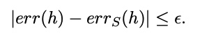
The relationship result by hoeffding bound

Let H be a finite hypothesis space. Let D be an arbitrary, fixed unknown probability distribution over X and let c ∗ be an arbitrary unknown target function. For any $\epsilon$, δ > 0, if we draw a sample S from D of size

image-20220402131238691

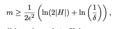
then probability at least (1 − δ), all hypotheses h in H have

image-20220402131254790

Proof: given a hypothesis h, by hoeffding boundinhg, we get that the probability that its observed error outside $\epsilon$ of its true error is at most

![Screen Shot 2022-04-02 at 3.54.11 PM](/figures/Screen Shot 2022-04-02 at 3.54.11 PM.png)

(based on hoeffding boudning, and the definition of $m$)

By union bound over all all h in H, we then get the desired result.

Infinite hophothesis set?

union bound is too loose! There may be many overlap between two hypothesises. That is, two hypothesises may label most data points the same.

Some definitions

  • The growth function of $H$ $g_H(m)$ is the maximum number of distinct labelling $H$ (a labelling for a $h \in H$ is just the results induced by $h$ for the given samples) can induce on any set $S$ of $m$ data points. (对于m个sample,最多能产生多少种label)

    • we say $H$ shatters(打碎) $S$ if $|H(S)| = 2^m$ , we assume this is a binary classification problem, i.e., the label is in {-1,1} (有这样一个m个sample,给任意一种label,都存在一个h可以产生这个label)

    • $g_H(m) = 2^m$ if exist S that H shatters it.

      ![Screen Shot 2022-04-02 at 11.54.20 PM](/figures/Screen Shot 2022-04-02 at 11.54.20 PM.png)

    • 2D linear seperator cannot shatter 4 points

    • D dimentional linear seperator can shatter D+1 points but cannot shatter D + 2 points

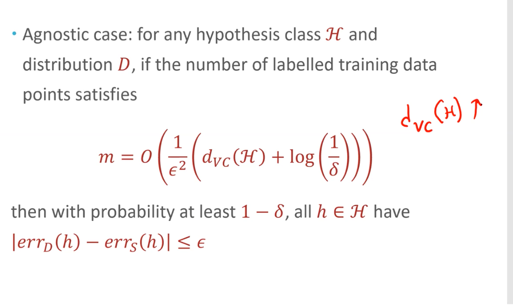
VC bound (relationship between data size and errors)

image-20220403000015185

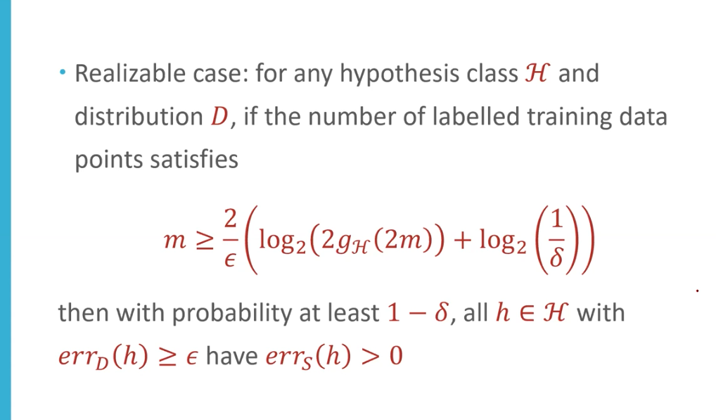
If no golden target:

image-20220403011338282

VC dimension (the complexity of the hyphothesis set)

$d_{VC}(H) = $ the largest value of $m$ s.t. $g_H(m) = 2^m$, i.e., the greatest number of data points that can be shattered by $H$

For example, for a N-dimensional linear seperator, its VC dimension is $D+1$

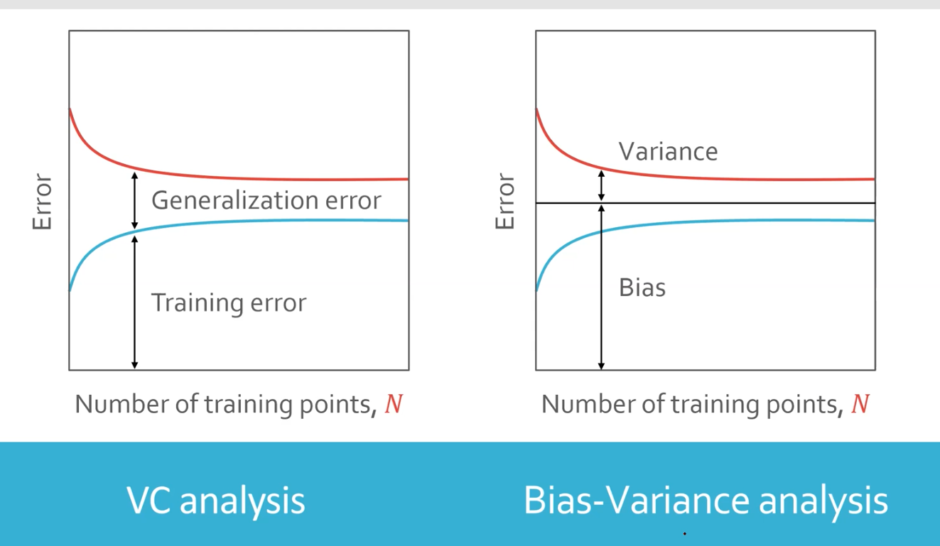
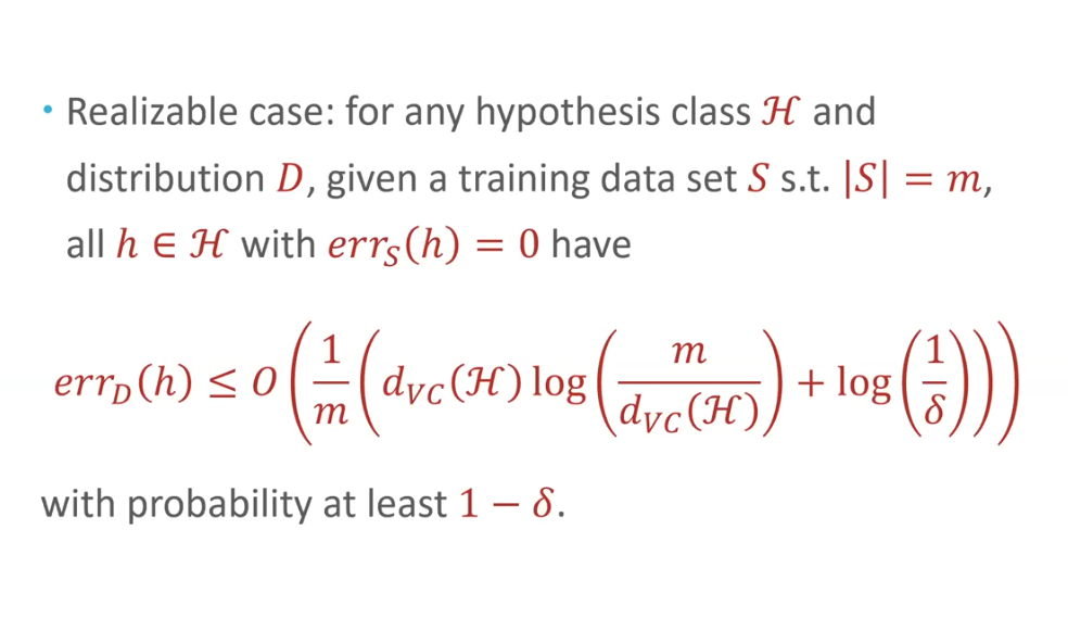
Statistical Learning Style bounds, (fixed data size,relationships between the true error and the data error)

image-20220403011717814

image-20220403011757356

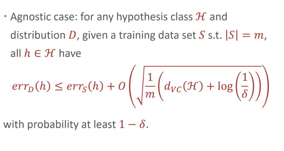
Agnostic case: trainning error is not zero

traning error decreases as VC dim increases (easier to )

the bound increases as VC dim increases (harder to generalize)

image-20220425114624651

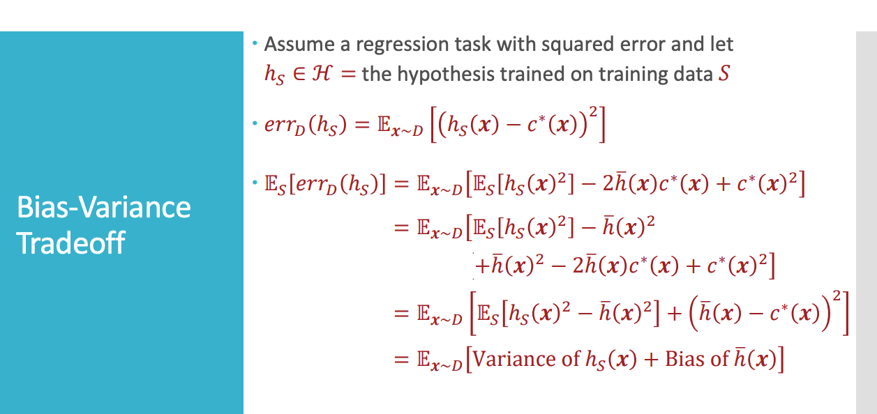
Two analysis illustration (VC analysis and bias-variance)

image-20220425162541501

GNNs for attacking

Now, all (at least from my knowledge) GNN-based works focus on attacking, that is, given a locked circuit, using GNNs to attack it (predict the correct key values).

These works can be roughly divided into two categories based on the target locking method.

To attack some logic locking methods, the problem can be formulated as a link prediction task. For example, for the MUX-based locking method, what the attacker is doing is actually trying to determine which edge in the MUX should be preserved.

Here are some papers (although most of them come from the same author)

  • ICCAD21 - UNTANGLE: Unlocking Routing and Logic Obfuscation Using Graph Neural Networks-based Link Prediction

  • DATE22 - MuxLink: Circumventing Learning-Resilient MUX-Locking Using Graph Neural Network-based Link Prediction

GNNs for node classification

  • DATE21- GNNUnlock: Graph Neural Networks-based Oracle-less Unlocking Scheme for Provably Secure Logic Locking
    • (Attack Anti-SAT) predict whether the node (gate) belongs to Anti-SAT (AN, green box) module or original design (DN, gray box)
    • image-20220508133120863
    • (TTLock and SFLL-HD) predict whether the node belongs to 1) orig design (DN) 2) pertub unit (PN) 3) restore unit (PN)
    • image-20220508171929174